Playing with Profile-Guided Optimization
Table of Contents
An optimizing compiler is one of the more impressive pieces of software most of us use every day. Between parsing your code and emitting instructions, clang will run it through a hundred-odd passes: inlining, loop transformations, vectorization, instruction selection, register allocation, block placement. Each of these passes rests on decades of research. It’s easy to treat the whole thing as a black box that turns C into something fast. Most of the time that’s fair.
The compiler does have one blind spot, though, and it’s built into the job. It has to produce one binary that’s correct for every input, and for most decisions it has no idea which inputs will actually show up. This post is about what that costs and how to hand the compiler the missing information.
What the compiler has to guess #
Take a branch like this one:
if (ins.flags & STAGE_3_RARE_CASE) {
    /* a dozen lines of fallback work */
}
To lay this out in memory, the compiler has to put one side of the branch straight after the test and jump to the other. One side becomes the fall-through path and the other becomes the taken jump. If the fall-through side is the common one, the CPU fetches straight-line code. If not, every execution pays for a taken branch, and the hot code ends up spread across more cache lines than it needs, interleaved with code that rarely runs.
Without more information, the compiler estimates branch probabilities from
static heuristics. Loop back-edges are probably taken. A comparison of a
pointer against null probably fails. A path that ends in a call to
abort() is probably cold. These rules work surprisingly well on typical
code. They have nothing to say about ins.flags & 8, which looks 50/50
to the compiler. Whether that bit is set 2% of the time or 98% of the
time depends on data the compiler never sees.
The usual manual escape hatch is __builtin_expect (or C++20’s
[[likely]]). It works, but it’s a hint written by a person, at the
time the code was written, about a workload that may since have changed.
And it only covers the branches someone thought to annotate.
Why it matters this much is a front-end story, covered in more detail in an earlier post on instruction cache pressure. A modern core can execute far more than it can fetch through a fragmented instruction stream. Taken branches cost fetch bandwidth. Code that’s hot but spread across many lines pushes other hot code out of the 32KB L1 instruction cache and out of the op cache. None of this shows up in an instruction count.
The obvious fix is to stop guessing and measure. Profile-guided optimization (PGO) does exactly that: build the program once with instrumentation, run it on a workload that looks like real use, and feed the recorded branch and call counts back into a second compile. The compiler makes the same decisions as before, but with measured numbers instead of heuristics. The idea is old - GCC has supported it for more than two decades - and the tooling is mature.
The three steps #
Taking clang as the target compiler, it’s three steps:
# 1. build with counters on every branch and call
clang -O2 -fprofile-generate -o app_instr app.c

# 2. run it on something representative; writes default_*.profraw
./app_instr typical-input

# 3. convert the raw counters, then rebuild using them
llvm-profdata merge -o app.profdata default_*.profraw
clang -O2 -fprofile-use=app.profdata -o app app.c
The instrumented build is noticeably slower, because every branch and call updates a counter. The training run only has to see the program’s behaviour; it doesn’t need to be long. Profiles from several runs can be merged in step 3.
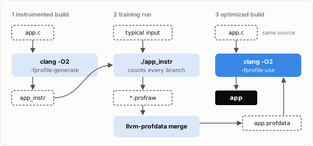
GCC has the same feature under the same flag names, with a different
profile format. Several large projects ship PGO builds: CPython’s
--enable-optimizations trains on its own test suite, Firefox and
Chrome are built with it, and GCC can build itself this way with
make profiledbootstrap.
What changes in the compiled code #
A profile turns guessed branch probabilities into measured ones, and every pass that consults them makes different decisions. The main ones:
- block placement. The hot path through each function becomes the fall-through path. Rarely executed blocks move to the end of the function, out of the way.
- inlining. Call sites that are executed often get a much larger inlining budget. Call sites that are never executed get none.
- register allocation. When something has to be spilled to the stack, spill and reload code lands on the cold paths.
- size versus speed. Functions that never ran in training are optimized for size, and hot and cold functions are grouped into separate sections, so the hot ones share fewer pages and cache lines.
The interesting consequence is that the code doesn’t only get rearranged. It’s different code: larger where the program spends its time and smaller everywhere else. That will show up in SQLite below.
A toy interpreter #
To isolate the effect, I wrote a small bytecode interpreter
(pgo-dispatch).
It’s a switch over 128 generated opcodes. Each opcode does eight
cheap steps, and after each step a bit in the instruction decides
whether to run a larger rare-case fragment:
case 17: {
    uint64_t a = r[3], b = r[9];
    a = (a ^ 0x9e3779b97f4a7c15ull) + (b >> 1) + ins.imm;
    if (ins.flags & 1) {
        /* six lines of rare-case arithmetic */
        a += b;
    }
    /* ... seven more steps like the first ... */
    r[5] = a ^ b;
    break;
}
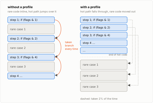
The shape is borrowed from real interpreters, where the fast path of an opcode is interleaved with type checks, overflow checks and error handling. The rare-case bits are set 2% of the time, but nothing in the source says so.
Without a profile, clang treats each of those checks as a coin flip and keeps the rare fragment where the source put it, right after the test. The hot path then jumps over every one of them. With a profile, the fragments move to the end of the function and the hot path becomes straight-line code:
Two workloads run on the same interpreter. Workload A only uses the first half of the opcodes and workload B only the second half; think of numeric code and string code in a scripting language. Within each half, opcode frequency is skewed, so a few opcodes are hot and most are warm. The program is built from short phrases that repeat, as real bytecode does. The phrases matter: with a random opcode stream, every dispatch is a mispredicted indirect jump, and that cost drowns out everything else.
I built it with plain -O2, then with PGO trained on A, on B, and on
both with the profiles merged. Each binary ran both workloads. All
variants are built without PIE, and every run produces the same
checksum. These numbers come from an AMD Ryzen 7 7840HS (Zen 4) with
clang 18, best of five runs:
| run on | trained on | time | taken branches | icache misses | speedup |
|---|---|---|---|---|---|
| A | - | 0.3302s | 651.4M | 22.9M | 1.00x |
| A | A | 0.2382s | 172.8M | 5.0M | 1.39x |
| A | B | 0.2840s | 646.4M | 17.7M | 1.16x |
| A | A+B | 0.2472s | 181.5M | 10.3M | 1.34x |
| B | - | 0.3057s | 643.4M | 21.6M | 1.00x |
| B | A | 0.2907s | 643.2M | 18.4M | 1.05x |
| B | B | 0.2388s | 174.0M | 5.2M | 1.28x |
| B | A+B | 0.2483s | 173.1M | 11.8M | 1.23x |
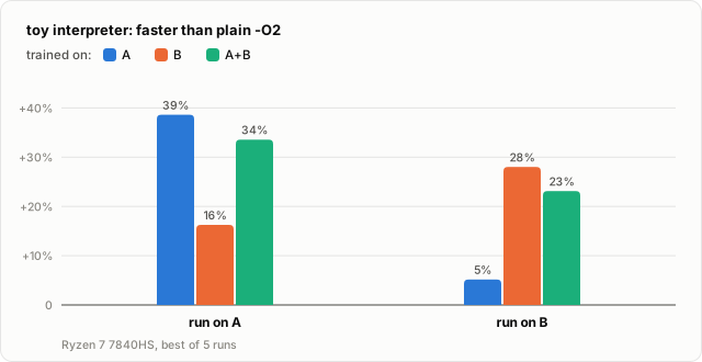
With a matching profile, the run gets 1.28–1.39x faster. Instructions retired go from 5.76G to 5.34G, a 7% drop that’s mostly the jumps that are no longer needed. That’s nowhere near enough to explain the speedup. The counters show where the rest comes from. Without a profile the interpreter takes about ten branches per opcode, one jump over each rare fragment plus the dispatch. With a matching profile it takes 2.6. Instruction cache misses fall by a similar factor of four, because the hot path of each opcode is now contiguous and the rare fragments no longer sit in the middle of it.
With the wrong profile, most of that disappears. The binary trained on B treats all of A’s opcodes as never executed, so none of the layout work lands where A needs it, and taken branches stay where they were. What’s left (1.16x on A, 1.05x on B) presumably comes from the cold half being compiled smaller, plus other second-order effects. I don’t have a clean explanation for why the leftover gain is asymmetric between the two directions.
The merged profile gets most of the benefit on both workloads. The icache column shows what it costs: twice as much code is treated as hot, and it all shares the same 32KB, so misses end up about double those of a matching profile.
SQLite #
A toy built to have this problem isn’t evidence that real code has it.
For a real program I used SQLite and its own benchmark, speedtest1
(bolt-sqlite).
That’s a reasonable candidate. Most of SQLite’s time goes into
sqlite3VdbeExec, a bytecode interpreter that is one large switch
over its roughly 190 opcodes. Around it sit a B-tree, a pager and a query
planner, all branchy, general-purpose code that has to handle every
schema and every query.
speedtest1 comes with several test sets, and I used four of them. These are the kinds of workload different users of the same library might have:
main: the default mix of inserts, indexed and unindexed selects, updates, deletes, joins and sortingorm: wide tables with machine-generated, ORM-style queriescte: recursive common table expressions, such as a sudoku solver and a Mandelbrot set written in SQLfp: floating-point values, conversions and aggregates
I trained PGO on main, on cte, and on both merged, at a quarter of
the benchmark size. Every binary ran all four test sets against an
in-memory database. All binaries produce the same result hash
(--verify).
Measured on the same machine as the toy, best of seven runs, taken
branches and icache misses from perf stat:
| test set | trained on | time | taken branches | icache misses | speedup |
|---|---|---|---|---|---|
| main | - | 1.750s | 2107.7M | 50.2M | 1.00x |
| main | main | 1.549s | 999.6M | 25.8M | 1.13x |
| main | cte | 1.659s | 1540.8M | 32.9M | 1.05x |
| main | main+cte | 1.559s | 1087.4M | 29.5M | 1.12x |
| orm | - | 0.775s | 1061.3M | 53.1M | 1.00x |
| orm | main | 0.716s | 696.9M | 34.2M | 1.08x |
| orm | cte | 0.752s | 827.0M | 38.6M | 1.03x |
| orm | main+cte | 0.702s | 709.0M | 33.9M | 1.10x |
| cte | - | 2.741s | 4569.0M | 43.6M | 1.00x |
| cte | main | 2.481s | 3229.6M | 33.9M | 1.10x |
| cte | cte | 2.284s | 2063.7M | 29.4M | 1.20x |
| cte | main+cte | 2.290s | 2171.7M | 35.7M | 1.20x |
| fp | - | 1.673s | 1879.9M | 15.5M | 1.00x |
| fp | main | 1.599s | 1450.8M | 13.3M | 1.05x |
| fp | cte | 1.628s | 1512.6M | 8.2M | 1.03x |
| fp | main+cte | 1.584s | 1417.9M | 13.3M | 1.06x |
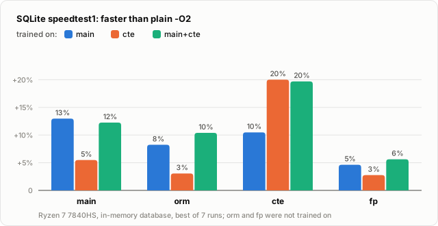
The pattern from the toy holds, at a smaller scale. A matching profile
gives 1.13x on main and 1.20x on cte. Training on the other test set
gives 1.05x and 1.10x, so less than half the gain carries over in one
direction and about half in the other. Taken branches tell the same
story: the main profile halves them on main, while the cte profile
removes only a quarter.
Neither orm nor fp was part of any training run, which makes them
the more honest test. Both gain from either profile, but the main
profile does better on both. main is the broader of the two training
workloads, and more of what it exercises is also what other workloads
use.
The merged profile is as good as the best single profile on every row,
within noise: 1.12x against 1.13x on main, and 1.20x on cte. It is
also the best of the three on both test sets that weren’t trained on.
Merging cost much less than in the toy, where the two workloads shared
no opcodes at all. Here the two profiles overlap heavily. The icache
column still shows the cost (35.7M misses against 29.4M on cte), but
it no longer shows up in the time.
The gains are smaller than in the toy, even when the counters move by similar factors. That’s expected: the toy was built so that nearly all of its time goes into fetching code, and SQLite does a fair amount of real work per branch.
A look inside #
It’s worth looking at what the profile did to the interpreter function itself (clang 18.1.8 builds; exact sizes vary between compiler versions):
| binary | sqlite3VdbeExec size | instructions | whole .text |
|---|---|---|---|
| base | 49.3KB | 11,229 | 1012KB |
| pgo-main | 79.7KB | 18,322 | 978KB |
| pgo-cte | 57.0KB | 13,261 | 882KB |
| pgo-main+cte | 109.5KB | 24,981 | 1021KB |
The hottest function grows, by 60% with the main profile, while the
program as a whole shrinks. Thirty-seven functions that the base build
calls from the interpreter loop are inlined into it in the pgo-main
build, among them sqlite3BtreeInsert, sqlite3PutVarint and
btreeGetPage. In the other direction, code that never ran in training
is compiled for size. With the cte profile, which exercises less of
SQLite, .text shrinks by 13%.
This also explains why a profile from one workload can still help a different one. Both profiles agree on a large common core: opening cursors, decoding records, comparing values, moving through B-tree pages. What they disagree about is how much of the code at the edges is hot.
Choosing what to train on #
Every result above comes down to the training run, which is the actual engineering problem in using PGO. Some observations from doing this:
- Train on what the program does in production, not on the benchmark. A narrow profile wins on the workload it was trained on and gives much less elsewhere. If you train on your benchmark, it will tell you the result you trained it to give.
- When in doubt, merge. A merged profile of several representative workloads gives up little or nothing on each of them, and in the SQLite runs it was the best choice for the workloads nobody trained on.
- Profiles go stale. A profile records counts against the code as it
was. When the code changes, clang matches what it can and ignores the
rest (
-Wprofile-instr-out-of-datetells you when this happens). The training run belongs in the build, not in a file committed once and forgotten. - The training run is part of the build. That means it needs to be deterministic enough to reproduce, and fast enough to run in CI. CPython’s test-suite training is a reasonable model.
An alternative to the instrumented build is sampling-based PGO
(AutoFDO in clang and GCC). Instead of a special build, you profile the
normal binary in production with perf, using the CPU’s branch
recording, and convert that into a profile for the next build. It’s
less precise, but the profile comes from real traffic instead of a
training script, which addresses the main weakness above.
Profiling as part of the build #
A profile describes the workload at one point in time, and workloads drift: users adopt new features, data grows, traffic shifts. A profile from last year can quietly optimize for a program that no longer runs. That’s the real argument for profiling periodically and proactively, not just once and not only when something is visibly slow - the same point the cache aliasing post ended on. With the training run in the build, every release gets a fresh profile, and a profile that changes noticeably from one release to the next is itself a signal that the workload has moved.
Conclusion #
PGO doesn’t make the compiler smarter. It gives the compiler a fact it can’t derive from the source: which way the branches actually go. For code limited by the front end, such as interpreters, databases, compilers and other large, branchy programs, that is worth 10–30% for the cost of one extra build and one training run. The part that takes real thought is choosing a training run that represents the program’s actual use.
The same information can also be applied later, to a binary that has already been linked, without rebuilding anything. That’s what LLVM’s BOLT does, and it’s the subject of the next post.
References #
- Clang - Profile Guided Optimization - the flags used here, and the sampling-based variant
- GCC - Instrumentation Options -
-fprofile-generateand-fprofile-usein GCC - SQLite - speedtest1 - the benchmark program
- darfire/bloggy-code - pgo-dispatch and bolt-sqlite - full code and
bench.shfor the numbers in this post